The Valve Wizard

Before reading this it is highly recommended that you read the section on the Single Ended Output Stage

When large amounts of output power are required (more than about 15W) the push-pull output stage becomes the order of the day. This arrangement allows the valves to be operated in Class AB, which is considerably more efficient than Class A (up to 80% compared with up to 50% respectively) reducing the amount of power wasted as heat in power valves. Not only this, but Class AB also allows us to operate the valves at much higher anode voltages and the load line can actually go beyond the maximum power dissipation curve. In this way the peak power level can actually exceed the combined maximum anode dissipation power of the two valves!

Of course, there is no reason why a push-pull stage cannot be operated in Class A, but this is rare in guitar amps since Class AB affords greater output power, and the output transformers are usually cheaper (and no, the Vox AC15/30 are NOT Class A amps!). Class A will have less headroom (i.e., will overdrive sooner) and zero crossover distortion in a like-for-like circuit. However, we can easily build a preamp capable of overdriving a Class AB stage, and crossover distortion is not particularly noticeable provided we do not operate very close to Class B.
A perfectly balanced push-pull stage will cancel all even harmonic distortion and sum odd harmonic distortion generated within the power stage. However, guitar amps rarely use matched valves and usually have a less-than-perfect phase inverter. (Even if the phase inverter is perfectly balanced it will inevitably go out of balance when the power stage is overdriven.) This is desirable for the retention of even order harmonics, providing distortion with both warmth and 'growl'.

Any valve textbook describing how to design a push-pull stage will explain how to draw 'composite characteristics'. These are simply the combined anode characteristics of the stage, as if the two valves in the circuit are rolled into one big valve (which as far as the output transformer is concerned, they are). Composite characteristics can be used to find precise values of distortion for a given load impedance, which is essential for hifi. However, in a guitar amp we do not need to find an "optimum load for minimum distortion" and we almost certainly won't be using matched valves. We simply want a stage that will work properly and sound good. More often than not we will be trying to pair up a power transformer and output transformer that have been scrounged, so this tutorial will outline the more simple method of designed a push-pull stage using load lines without the rigmarole of drawing composite characteristics.

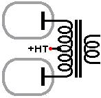An output transformer designed for push-pull operation has a centre tap. The HT is applied to the centre tap and either end of the primary winding is connected to the anode of a power valve. In this way, current flows in opposite directions through the output transformer. If these currents are equal they will cancel out and this is why push-pull output transformers can be made much smaller than single ended ones with the same power rating- there is (almost) no standing current in the transformer so no air gap and less iron is required.
The valves are driven with identical but out-of-phase grid signals. When one grid goes positive, the other goes negative. When one valves conducts more, the other conducts less: one pushes, the other pulls. The output signal developed in the transformer is the difference between the two AC currents.

Because the stage is symmetrical we can ignore one side of it and concentrate on drawing load lines for just one valve, then simply duplicate what we find for the other valve.
Usually we have a rough idea of the HT voltage we will be using, and probably an output transformer to hand already. What we would like to know is what class will it be operating in, how should we bias the valves, and possibly; how much output power can we expect? Of course, the whole method can be worked backwards to find a suitable transformer or HT voltage etc., as you see fit.

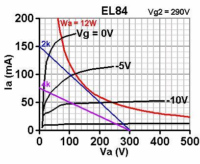
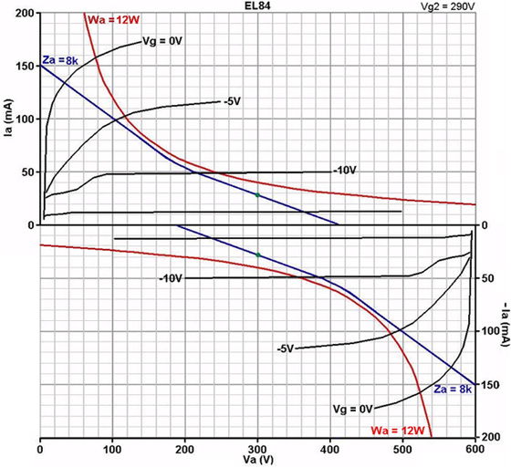
In the following example we will design a stage for a pair of EL84's with an HT of 300V and an 8k anode-to-anode primary impedance. A glance at some example values on the data sheet would tell you that this particular voltage and impedance are more-or-less suitable for use with EL84's.

The question is often asked; "what load do the valves 'see' in Class AB?". The answer lies in the name 'Class AB' - a combination of Class A and Class B.
While both valves are conducting the amplifier operates in Class A, and both valves 'see' a load of ½ the anode-anode impedance of the transformer (1/2 Za-a). However, as soon as one valve cuts off, that half of the transformer's primary is no longer part of the circuit. Because the impedance ratio is the square of the turns ratio, the load presented to the remaining 'on' valve must be only ¼ Za-a. So the stage operates in Class B at higher signal levels. Drawing a load line to show this is simple:

First draw a load line corresponding to ¼ Za-a. In this case that is ¼ 8k = 2k. This is the Class B part of the load [blue line in the image above].
This line may pass above the 'knee' of the grid curves for triode-like operation (good for hifi).
It may pass through the knee, which gives maximum power efficiency and is what the textbooks will tell you to do.
It may slightly pass below the knee. This is typical of guitar amps, but we must ensure that, during operation, the screen voltage can 'sag' so that as the operating point moves towards the left, the grid curves are pulled down so the line ends up passing through or above the knee. 1k screen stopper resistors are normally sufficient to acheive this.
If your line passes a long way below the knee, then the screen voltage must be lowered, or a very sizeable screen-grid stopper must be used. See the section on the pentode on how to do this. This load line may cross the max dissipation curve over a portion of its length- this is allowable.
Second, draw a load line corresponding to ½ Za-a. In this case it is ½ 8k = 4k. This is the Class A part of the load [purple line]. But as it stands, we appear to have biased the stage just to the point of cut-off, so it is only Class B.

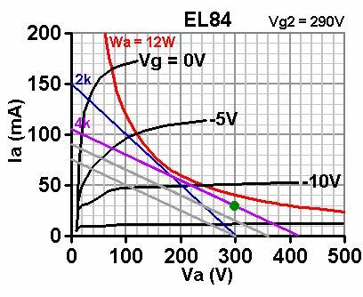To push the stage into Class AB we slide the Class A load line up the graph while maintaining its gradient, in exactly the same way as for the Single Ended Output Stage and see what bias voltage is required, the grey lines show this process. In fact, this is what we are doing whenever we adjust the bias on a fixed-bias amp! If we bias hot enough (i.e., push the Class A load line up far enough) it will become pure ClassA.
Of course, the bias point must not be pushed above the maximum dissipation curve, and it is usual to bias well under it to avoid damage (70% of maximum dissipation is often recommended, although anything up to about 85% would be ok).
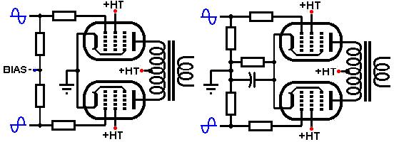
The load line indicates we need roughly 12V bias voltage. This can either be provided via a cathode bias resistor [below right], or by applying a fixed negative voltage to the grid [below left]. If using cathode bias, each valve can be given its own bias resistor and capacitor, or they can both share the same one (of half the resistance, twice the power rating), which tends to encourage extra second harmonic distortion [below right].
Cathode bias often lends a natural compression or 'squishiness' to the sound, due to the increase in bias voltage when one valve enters Class B conditions, though the larger the bypass capacitor, the less will be this effect. A small capacitor (less than 100uF say) also increases non-linear distortion, which may be significant in hifi. Using a very large capacitor (greater than 470uF say), or using no capacitor at all, reduces this effect.
Fixed bias on the other hand, remains the same at all times. This allows maximum output power to be developed, and the reduced compression gives faithful transient response, or a stiff or 'barking' overdriven sound.
Furthermore, there is no reason why we cannot use a little fixed bias and cathode bias simultaneously to achieve the desired mix of compression and 'bark'.

Owing to the "bunching" of the grid curves in each valve, the transition from Class A to B conditions is not abrupt, but a smooth curve. Note also that while the stage operates in Class A, current drawn from the power supply is constant. Once one valve enters Class B, the current demand increases- this is what causes power supply 'sag' when a valve rectifier is used. It is this 'boost' in current that compensates for the fact that one valve is no longer amplifying at all. The final load line is shown below, with the identical one for the second valve in the pair 'mirroring it', in anti-phase.

Output power:
The total output power can be closely estimated from the load line (again, we only need to look at one half of the circuit to do this).
Simply note the peak current Ipeak (i.e., where the load line crosses the 0V grid curve); in this case it is about 135mA. Also note the minimum anode voltage Vmin, which is about 35V in this case. The total (rms) output power is then approximately:
P = (HT-Vmin) * Ipeak / 2
P = (300-35) * 0.135 / 2
= 17.9W
Even without a load line you can estimate the output power for a typical pentode, assuming the load impedance isn't unusually small for the type of valve being used:
P = 2 * (HT-50)^2 / Rload
Where Rload is the anode-to-anode impedance of the transformer. The '50' in the above equation is an estimation of how low the anode voltage can swing in a typical pentode/tetrode. In this case we would have predicted a value of 15.6W, which is not much less than what load line is saying.